Vector Search Fundamentals: Embeddings, Similarity Metrics, and Approximate Nearest Neighbors

Traditional search matches keywords. Users must know the exact words in the documents they seek. Vector search matches meaning. Users describe what they are looking for in natural language, and the system finds semantically similar content even when keywords differ. “Car trouble” finds documents about “automotive repair” and “engine problems.”

Vector search powers modern semantic search, recommendation systems, and retrieval-augmented generation (RAG) for LLMs. It converts text, images, or other content into high-dimensional vectors (embeddings) that capture semantic meaning. It then searches for vectors most similar to a query vector using specialized algorithms that find approximate nearest neighbors efficiently at scale.

I have built vector search systems for knowledge bases, product catalogs, and content recommendation. I have learned that embedding model selection dramatically impacts quality, that similarity metric choice affects results, and that approximate nearest neighbor (ANN) algorithms enable search at million-document scale. This guide covers the patterns that work: understanding embeddings and their properties, similarity metrics and when to use each, ANN algorithms that make vector search practical, vector database selection, and building complete semantic search pipelines.

Understanding Embeddings

What Are Embeddings

Embeddings are dense numerical vectors that represent semantic meaning. Similar items have similar vectors.

Text: "The quick brown fox"
Embedding: [0.12, -0.45, 0.89, ..., 0.34]  # 384 to 1536 dimensions

Text: "A fast brown animal"
Embedding: [0.14, -0.42, 0.87, ..., 0.31]  # Similar vector

Text: "Quantum computing"
Embedding: [-0.78, 0.23, -0.12, ..., 0.91]  # Very different vector

Properties of Good Embeddings

Semantic similarity: Similar meaning = close in vector space

Linear relationships: Analogies work as vector arithmetic

king - man + woman ≈ queen
Paris - France + Italy ≈ Rome

Dense representation: All dimensions have values (vs sparse one-hot encoding)

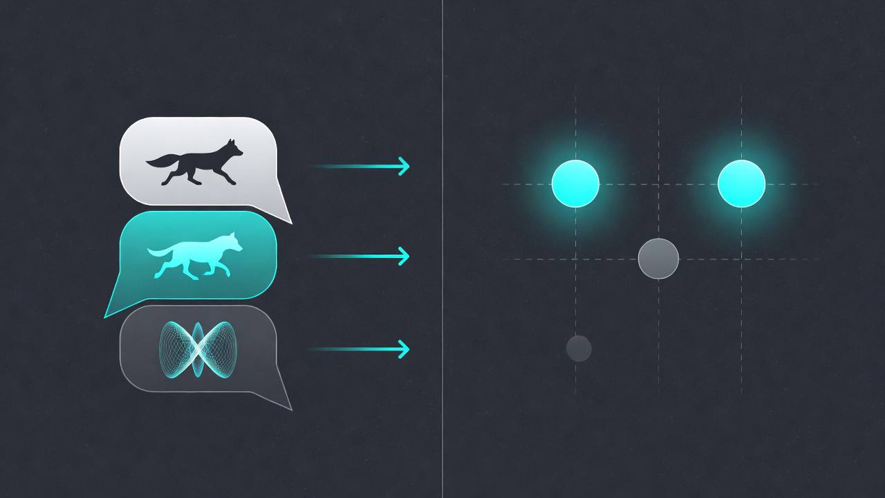Similar meanings produce vectors that cluster together in high-dimensional space.

Embedding Models

Text embedding models:

Model	Dimensions	Best For	Provider
text-embedding-3-small	1536	General purpose	OpenAI
text-embedding-3-large	3072	High accuracy	OpenAI
text-embedding-ada-002	1536	Legacy	OpenAI
sentence-transformers/all-MiniLM	384	Cost-effective	Open source
sentence-transformers/all-mpnet-base	768	Balanced	Open source
voyage-2	1024	High quality	Voyage AI
Cohere embed	1024	Multilingual	Cohere

Selection criteria:

• Quality: Benchmark on your specific data
• Cost: API costs or compute for self-hosted
• Dimensions: Higher dimensions = more accurate but more storage
• Latency: Model inference time

Generating Embeddings

# OpenAI
from openai import OpenAI

client = OpenAI()

def get_embedding(text: str, model: str = "text-embedding-3-small") -> list[float]:
    # Replace newlines, which can affect results
    text = text.replace("\n", " ")
    
    response = client.embeddings.create(
        input=text,
        model=model
    )
    
    return response.data[0].embedding

# Batch processing for efficiency
async def get_embeddings_batch(texts: list[str], batch_size: int = 100) -> list[list[float]]:
    embeddings = []
    
    for i in range(0, len(texts), batch_size):
        batch = texts[i:i + batch_size]
        response = await client.embeddings.create(input=batch, model="text-embedding-3-small")
        embeddings.extend([item.embedding for item in response.data])
    
    return embeddings

# Open source (sentence-transformers)
from sentence_transformers import SentenceTransformer

model = SentenceTransformer('all-MiniLM-L6-v2')

def get_embedding(text: str) -> list[float]:
    embedding = model.encode(text)
    return embedding.tolist()

# Batch processing
embeddings = model.encode(texts, batch_size=32, show_progress_bar=True)

For teams evaluating whether to run embeddings locally or via API, cost and latency tradeoffs matter. Our guide to locally run AI breaks down when self-hosting saves money versus using managed embedding APIs.

Similarity Metrics

Cosine Similarity

Measures angle between vectors, ignoring magnitude.

import numpy as np

def cosine_similarity(a: np.ndarray, b: np.ndarray) -> float:
    return np.dot(a, b) / (np.linalg.norm(a) * np.linalg.norm(b))

# Ranges from -1 (opposite) to 1 (identical)
# Most common for text embeddings

When to use:

• Text embeddings (most models normalized)
• When direction matters more than magnitude
• Most common default choice

Euclidean Distance

Straight-line distance between vectors.

def euclidean_distance(a: np.ndarray, b: np.ndarray) -> float:
    return np.linalg.norm(a - b)

# Lower = more similar

When to use:

• When magnitude matters
• Computer vision embeddings
• When vectors are not normalized

Dot Product

Simple sum of element-wise products.

def dot_product(a: np.ndarray, b: np.ndarray) -> float:
    return np.dot(a, b)

When to use:

• When vectors are normalized (equivalent to cosine)
• Fast computation
• Some vector databases optimize for this

Metric Selection Guide

Metric	Use When	Range
Cosine	Text search, normalized vectors	[-1, 1]
Euclidean	Magnitude matters, vision	[0, ∞)
Dot Product	Normalized vectors, speed	(-∞, ∞)

Approximate Nearest Neighbor (ANN) Algorithms

Why ANN

Exact nearest neighbor search is O(n) with high dimensional data. At million-document scale, it is too slow.

ANN algorithms trade small accuracy loss for massive speed gains (1000x+).

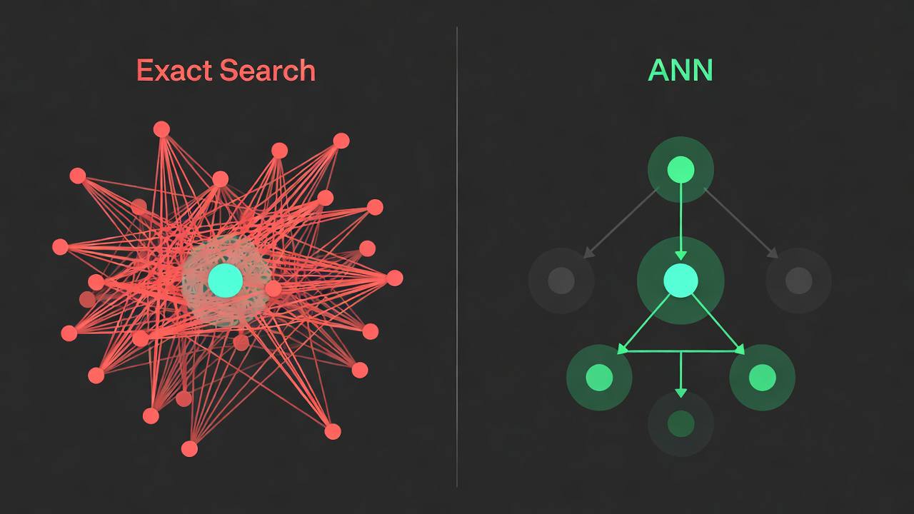ANN algorithms build hierarchical graphs that navigate directly to the most similar vectors without scanning every entry.

HNSW (Hierarchical Navigable Small World)

Graph-based algorithm. Most popular for production.

Building:
1. Insert points into layered graph structure
2. Each layer is a proximity graph
3. Top layer is sparse, lower layers denser

Searching:
1. Start at random point in top layer
2. Greedy walk to closest point
3. Drop to lower layer when local minimum reached
4. Repeat until bottom layer

Characteristics:

• High recall (typically >95%)
• Fast queries (milliseconds)
• Memory intensive (stores graph)
• Good for million-scale datasets

IVF (Inverted File Index)

Clustering-based approach.

Building:
1. Cluster vectors into N groups (voronoi cells)
2. Store cluster centroids

Searching:
1. Find nearest cluster centroids to query
2. Search only vectors in those clusters
3. Refine with exact search on candidates

Characteristics:

• Tunable speed/accuracy tradeoff
• Memory efficient
• Good for billion-scale datasets

LSH (Locality Sensitive Hashing)

Hash-based approach.

Building:
1. Create multiple hash functions
2. Similar vectors hash to same buckets

Searching:
1. Hash query vector
2. Check all vectors in matching buckets
3. Refine with exact similarity

Characteristics:

• Very fast
• Lower recall than HNSW
• Good for very large datasets where recall can be lower

PQ (Product Quantization)

Compression technique often combined with other indexes.

Compress vectors by:
1. Split vector into sub-vectors
2. Quantize each sub-vector to a codebook
3. Store codes instead of full vectors

Enables:
- 10-20x memory reduction
- Faster distance computation
- Slight accuracy loss

Vector Databases

Pinecone

Pinecone is a managed vector database.

from pinecone import Pinecone, ServerlessSpec

pc = PineCone(api_key="your-api-key")

# Create index
pc.create_index(
    name="my-index",
    dimension=1536,  # Matches embedding model
    metric="cosine",
    spec=ServerlessSpec(cloud="aws", region="us-east-1")
)

index = pc.Index("my-index")

# Upsert vectors
index.upsert(
    vectors=[
        {
            "id": "doc1",
            "values": embedding,
            "metadata": {"source": "article1", "category": "tech"}
        }
    ]
)

# Query
results = index.query(
    vector=query_embedding,
    top_k=10,
    filter={"category": {"$eq": "tech"}},
    include_metadata=True
)

Weaviate

Weaviate is an open-source vector database with a managed option.

import weaviate

client = weaviate.Client("http://localhost:8080")

# Create schema
class_obj = {
    "class": "Article",
    "vectorizer": "text2vec-openai",
    "moduleConfig": {
        "text2vec-openai": {
            "vectorizeClassName": False
        }
    },
    "properties": [
        {"name": "title", "dataType": ["text"]},
        {"name": "content", "dataType": ["text"]},
        {"name": "category", "dataType": ["text"]}
    ]
}

client.schema.create_class(class_obj)

# Insert (automatically vectorized)
client.data_object.create(
    data_object={
        "title": "Vector Search Guide",
        "content": "Content here...",
        "category": "tech"
    },
    class_name="Article"
)

# Query
result = (
    client.query
    .get("Article", ["title", "content"])
    .with_near_text({"concepts": ["semantic search"]})  # Auto-vectorized
    .with_limit(10)
    .do()
)

pgvector

pgvector is a PostgreSQL extension that adds vector similarity search to existing Postgres databases.

-- Enable extension
CREATE EXTENSION vector;

-- Create table
CREATE TABLE documents (
    id SERIAL PRIMARY KEY,
    content TEXT,
    embedding VECTOR(1536)
);

-- Create index
CREATE INDEX ON documents 
USING ivfflat (embedding vector_cosine_ops)
WITH (lists = 100);

-- Insert
INSERT INTO documents (content, embedding)
VALUES ('text here', '[0.1, 0.2, ...]');

-- Query
SELECT content, 1 - (embedding <=> query_embedding) AS cosine_similarity
FROM documents
ORDER BY embedding <=> query_embedding
LIMIT 10;

# Using with SQLAlchemy
from sqlalchemy import create_engine, Column, Integer, String
from pgvector.sqlalchemy import Vector

class Document(Base):
    __tablename__ = 'documents'
    
    id = Column(Integer, primary_key=True)
    content = Column(String)
    embedding = Column(Vector(1536))

# Query
docs = session.query(Document).order_by(
    Document.embedding.cosine_distance(query_embedding)
).limit(10).all()

Selection Guide

Database	Best For	Deployment
Pinecone	Managed, easy start	SaaS
Weaviate	Flexibility, features	Self-hosted or SaaS
pgvector	Existing Postgres	Self-hosted
Milvus	High scale, hybrid search	Self-hosted or SaaS
Chroma	Local development, simplicity	Embedded
Qdrant	Rust-based, fast	Self-hosted or SaaS

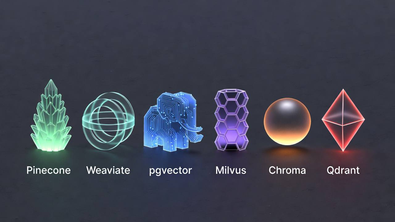Each vector database optimizes for different deployment models and scale requirements.

Building a Semantic Search Pipeline

Architecture

Documents
    |
    v
Chunking → Embedding → Vector DB
                              |
Query → Embedding → Similarity Search → Reranking → Results

Chunking Strategy

def chunk_text(text: str, chunk_size: int = 500, overlap: int = 50) -> list[str]:
    """Chunk text with overlap for context preservation"""
    chunks = []
    start = 0
    
    while start < len(text):
        end = start + chunk_size
        chunk = text[start:end]
        
        # Try to end at sentence boundary
        if end < len(text):
            last_period = chunk.rfind('.')
            if last_period > chunk_size * 0.7:  # If found in last 30%
                chunk = chunk[:last_period + 1]
                end = start + len(chunk)
        
        chunks.append(chunk.strip())
        start = end - overlap  # Overlap for context
    
    return chunks

# Semantic chunking with embeddings
def semantic_chunk(text: str, similarity_threshold: float = 0.8) -> list[str]:
    """Chunk based on semantic similarity"""
    sentences = text.split('. ')
    chunks = []
    current_chunk = [sentences[0]]
    
    for i in range(1, len(sentences)):
        prev_embedding = get_embedding(sentences[i-1])
        curr_embedding = get_embedding(sentences[i])
        
        similarity = cosine_similarity(prev_embedding, curr_embedding)
        
        if similarity > similarity_threshold:
            current_chunk.append(sentences[i])
        else:
            chunks.append('. '.join(current_chunk))
            current_chunk = [sentences[i]]
    
    if current_chunk:
        chunks.append('. '.join(current_chunk))
    
    return chunks

Hybrid Search

Combine vector similarity with keyword matching.

def hybrid_search(query: str, vector_weight: float = 0.7) -> list[dict]:
    """Combine BM25 and vector search"""
    
    # Vector search
    query_embedding = get_embedding(query)
    vector_results = vector_db.search(query_embedding, k=100)
    
    # Keyword search
    keyword_results = keyword_index.search(query, k=100)
    
    # Reciprocal Rank Fusion
    scores = {}
    
    for rank, result in enumerate(vector_results):
        doc_id = result['id']
        scores[doc_id] = scores.get(doc_id, 0) + vector_weight / (rank + 60)
    
    for rank, result in enumerate(keyword_results):
        doc_id = result['id']
        scores[doc_id] = scores.get(doc_id, 0) + (1 - vector_weight) / (rank + 60)
    
    # Sort by fused score
    ranked = sorted(scores.items(), key=lambda x: x[1], reverse=True)
    
    return [get_document(doc_id) for doc_id, _ in ranked[:10]]

Reranking

Initial retrieval (fast, approximate) → Reranking (slower, accurate).

def search_with_reranking(query: str) -> list[dict]:
    # Initial retrieval (ANN)
    query_embedding = get_embedding(query)
    candidates = vector_db.query(query_embedding, top_k=100)
    
    # Rerank with cross-encoder (more accurate)
    from sentence_transformers import CrossEncoder
    
    reranker = CrossEncoder('cross-encoder/ms-marco-MiniLM-L-6-v2')
    
    pairs = [[query, candidate['text']] for candidate in candidates]
    scores = reranker.predict(pairs)
    
    # Sort by reranker score
    for candidate, score in zip(candidates, scores):
        candidate['rerank_score'] = score
    
    reranked = sorted(candidates, key=lambda x: x['rerank_score'], reverse=True)
    
    return reranked[:10]

Filtering and Metadata

# Pinecone with metadata filter
results = index.query(
    vector=query_embedding,
    top_k=10,
    filter={
        "category": {"$eq": "documentation"},
        "created_at": {"$gte": "2024-01-01"},
        "$or": [
            {"author": {"$eq": "team-a"}},
            {"author": {"$eq": "team-b"}}
        ]
    }
)

Performance Optimization

Index Tuning

# HNSW parameters
index_params = {
    "M": 16,        # Connections per layer (higher = more accurate, more memory)
    "efConstruction": 200,  # Size of dynamic candidate list during construction
    "ef": 100       # Size of dynamic candidate list during search
}

# Tradeoffs:
# M: 8-64 (default 16). Higher = better recall, more memory
# efConstruction: 64-512. Higher = better index quality, slower build
# ef: 16-512. Higher = better recall, slower queries

Batch Operations

# Batch embedding (much faster)
texts = [doc['content'] for doc in documents]
embeddings = model.encode(texts, batch_size=64)

# Batch upsert
vectors_to_upsert = [
    {
        "id": doc['id'],
        "values": embedding.tolist(),
        "metadata": {"source": doc['source']}
    }
    for doc, embedding in zip(documents, embeddings)
]

# Upsert in batches
for i in range(0, len(vectors_to_upsert), 100):
    batch = vectors_to_upsert[i:i+100]
    index.upsert(vectors=batch)

Caching

from functools import lru_cache

@lru_cache(maxsize=10000)
def get_cached_embedding(text: str) -> tuple[list[float], str]:
    """Cache embeddings by text hash"""
    embedding = get_embedding(text)
    return tuple(embedding)  # Must be hashable for cache

Evaluation

Metrics

def evaluate_search(queries: list[dict]) -> dict:
    """
    queries: [{"query": str, "relevant_ids": [str]}]
    """
    results = {
        'recall@10': [],
        'precision@10': [],
        'mrr': [],
        'ndcg': []
    }
    
    for q in queries:
        search_results = search(q['query'], k=10)
        retrieved_ids = [r['id'] for r in search_results]
        relevant_ids = set(q['relevant_ids'])
        
        # Recall@10
        recall = len(relevant_ids & set(retrieved_ids)) / len(relevant_ids)
        results['recall@10'].append(recall)
        
        # Precision@10
        precision = len(relevant_ids & set(retrieved_ids)) / len(retrieved_ids)
        results['precision@10'].append(precision)
        
        # MRR
        for rank, doc_id in enumerate(retrieved_ids, 1):
            if doc_id in relevant_ids:
                results['mrr'].append(1 / rank)
                break
        else:
            results['mrr'].append(0)
    
    return {
        'recall@10': np.mean(results['recall@10']),
        'precision@10': np.mean(results['precision@10']),
        'mrr': np.mean(results['mrr'])
    }

Common Pitfalls

Pitfall 1: Wrong Embedding Model

Using general embeddings for domain-specific content. Use domain-tuned models.

Pitfall 2: Poor Chunking

Chunks that break semantic coherence. Use overlap and semantic boundaries.

Pitfall 3: No Metadata Filtering

Searching across all documents when users need filtered results. Index metadata.

Pitfall 4: Ignoring Exact Matches

Relying only on vectors when users search for specific IDs or names. Use hybrid search.

Pitfall 5: Wrong Similarity Metric

Using Euclidean distance on normalized embeddings. Use cosine for text.

Pitfall 6: Not Monitoring Quality

Search quality degrades over time without measurement. Evaluate regularly.

Conclusion

Vector search enables semantic understanding at scale. Choose embedding models that match your domain and quality requirements. Select similarity metrics appropriate for your embeddings. Use ANN algorithms for production-scale performance. Consider vector databases based on your operational requirements.

Build complete pipelines with proper chunking, hybrid search for best results, and reranking for precision. Monitor quality metrics and iterate.

Vector search is foundational technology for modern AI applications. Master it to build systems that understand user intent, not just match keywords. For teams building production AI systems, understanding how to cut LLM costs without sacrificing quality and protecting against prompt injection attacks are the next logical steps after getting search working.

---

Further Reading

• Pinecone documentation: Vector search tutorials and API reference
• Weaviate documentation: Vector database guides and schema design
• pgvector GitHub repository: PostgreSQL vector extension source and docs
• ANN Benchmarks: Comprehensive algorithm comparison across datasets
• Sentence Transformers documentation: Embedding models and training guides
• HNSW paper (Malkov & Yashunin, 2016): Algorithm fundamentals and performance analysis
• OpenAI Embeddings Guide: Best practices for text embedding generation
• MTEB Leaderboard: Massive Text Embedding Benchmark rankings